What is Support Vector Machine in Data Science?

Data science is a field that deals with extracting meaningful insights from large datasets. One of the most popular techniques used in data science is machine learning, which involves training algorithms to make predictions or decisions based on past data. Support vector machines (SVM) are one such algorithm that has gained popularity due to their ability to handle complex datasets and produce accurate results.

This blog post will discuss what support vector machines are and how they work. We will also explore two types of SVMs - positive support vector machines and negative support vector machines - and their applications in real-world scenarios. Understanding support vector machine in data mining begins with understanding data science; you can get an insight into the same through our Data Science Training.  

What are Support Vector Machines?

The support vector machine, also known as SVM, is a well-known approach to supervised learning that may be utilized for classification and regression work. However, its main application is in the field of machine learning, namely in the area of classification problems, where it is utilized.

The goal of the Support Vector Machine (SVM) technique is to locate the best line or decision boundary that may be used to partition the n-dimensional space into classes in a way that facilitates the uncomplicated classification of the following data points. For the purpose of describing this optimal decision boundary, hyperplanes are used.

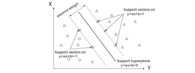
The selection of the hyper-extreme points and vectors is what the SVM does in order to generate the hyperplane. These types of corner situations are referred to as support vectors, and the technique that corresponds to them is referred to as a support vector machine. Take a look at the following picture, which presents an example of how a decision boundary (also known as a hyperplane) can be used to differentiate between two different groups:

Positive Support Vector Machine

A positive support vector machine (PSVM) is an extension of standard SVM designed for imbalanced datasets where one class has significantly fewer instances than others.In PSVM, instead of maximizing overall accuracy like regular SVMs do, it aims at maximizing precision for minority class samples while maintaining high recall rates across all classes.This approach helps reduce false positives while increasing true positives for underrepresented classes leading to better model performance on imbalanced datasets.PSVM can be helpful in various applications, such as fraud detection or disease diagnosis, where rare events need more attention than common ones.

Negative Support Vector Machine

A negative support vector machine (NSVM) is another extension of SVM designed for one-class classification problems where only positive examples are available and negative ones are unknown or irrelevant.In NSVM, the algorithm learns to identify the boundaries of the positive class by maximizing the margin around it while ignoring any other data points that do not belong to this class.This approach can be useful in anomaly or outlier detection tasks where identifying rare events is more important than finding normal patterns. It can also be used in image segmentation or text categorization applications.

History of Support Vector Machine

By using Support Vector Machines, a novel approach has been developed that may be used to classify both linear and nonlinear data. A support vector machine (SVM) is a type of machine learning method that, in brief, does the following. The training set is up-dimensionalized through nonlinear mapping. Specifically, it looks for the linear optimum separation hyperplane (a "decision border" dividing tuples into classes) inside this additional space. Whenever there are two classes of data, they may always be divided by a hyperplane if the nonlinear mapping is performed to a sufficiently high dimension. Using margins and support vectors ("essential" training tuples), the SVM determines the location of this hyperplane (defined by the support vectors). Even additional exploration of these novel ideas is forthcoming.

Although the foundation for SVMs (including early work by Vapnik and Alexei Chervonenkis on statistical learning theory) dates back to the 1960s, the first article on support vector machines was presented in 1992 by Vladimir Vapnik, Bernhard Boser, and Isabelle Guyon. Due to their capacity to simulate complicated nonlinear decision boundaries, SVMs are very accurate, despite the fact that even the fastest SVMs can take a long time to train. Overfitting is significantly less of an issue when using them.

Types of Support Vector Machine

The Support vector machine(SVM) can be classified into two categories:

1. Linear Support Vector Machine: If a dataset can be split into two groups along a straight line, we say it is linearly separable. We employ a Linear Support Vector Machine (SVM) classifier for such data.

2. Non-Linear Support Vector Machine: When a dataset cannot be categorized along a straight line, it is said to be non-linear, and the classifier employed in such cases is known as a non-linear support vector machine (SVM).

The SVM Algorithm's Hyperplane and Support Vectors:

Hyperplane:

In n-dimensional space, several possible lines (decision boundaries) may divide the space into distinct classes; nonetheless, it is necessary to choose the line that provides the most accurate classification of the data. The optimal boundary is represented as a hyperplane of SVM.

If there are only two characteristics (as seen in the illustration), then the hyperplane will be a straight line since those features determine its dimensions. Furthermore, if there are three characteristics, the hyperplane will be a flat, two-dimensional surface.

We always generate a hyperplane with the largest possible margin or the greatest possible separation between the data points.

Support Vectors:

What we call "Support Vectors" are the vectors or data points closest to the hyperplane and hence have the greatest influence on its location. These vectors are known as support vectors because they maintain the hyperplane.

What is Support Vector Machines Working

Let's start with the simplest possible example, a two-class problem where the classes can be separated in a linear way to figure out how SVMs work. To illustrate, suppose we have a dataset D represented as (X1, y1), (X2, y2),... (X|D|, y|D|), where Xi is a collection of training tuples that includes the class label yi.

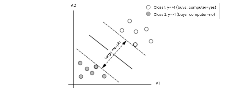
The classes "buy computer = yes and buys computer = no correspond to the possible values of +1 and -1 for yi, respectively. Let's look at the Figure below to understand better the relationship between the two input qualities A1 and A2.

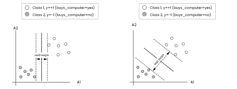
Because a straight line can be drawn to divide all the tuples in class +1 from all the tuples in class -1, it is clear that the 2-D data are linearly separable (or "linear," for short). The number of possible dividing lines is unlimited. To this end, we're looking for the "best" candidate or the one that (ideally) produces the smallest amount of misclassification for new tuples. Remember that if our data were three-dimensional (i.e., had three qualities), we would seek the most suitable splitting plane. In n dimensions, generally, we seek the optimal hyperplane. The decision boundary will be referred to as a "hyperplane" in this paper, regardless of the number of input characteristics. In other words, what is the best way to locate a suitable hyperplane?

An SVM tackles this issue by looking for the largest marginal hyperplane. Look at the figure above, which depicts two different hyperplanes and their respective boundaries. Let's take a quick hunch-based look at this graph before we understand the technical definition of margins. Both hyperplanes may properly categorize all possible pairs of data. The greater margin hyperplane is intuitively expected to perform better at categorizing future data tuples. For this reason, the SVM looks for the hyperplane with the biggest margin (the maximum marginal hyperplane) during the learning or training phase (MMH). Maximum differentiation across groups is represented by the boundary thus related. The "sides" of a margin are parallel to the hyperplane. Therefore, the shortest distance from the hyperplane to one side of its margin equals the shortest distance from the hyperplane to the other side. Given the MMH, this is the nearest training tuple of either class and hence the smallest distance possible.

The equation for a separating hyperplane is 

W*X +b = 0,
where W is a weight vector (W = w1, w2,..., wn),
X is an attribute space, and 
b is a scalar (also called a bias). 

Consider two input qualities, A1 and A2, as shown above, to make this easier to understand. For example, a 2-dimensional training tuple might look like X = (x1, x2), where x1 and x2 are the values of attributes A1 and A2 for X. When b is added to the aforementioned separating hyperplane, the new equation reads w0 + w1x1 + w2x2 = 0.

Therefore, if a point is located above the dividing hyperplane, then 

w0 + w1x1 + w2x2 > 0.

The same holds true for the separation hyperplane: every point below it must have the condition w0 + w1x1 + w2x2 0.

When the weights are set up properly, the hyperplanes that define the "sides" of the margin may be expressed as 

H1: w0 +w1x1 +w2x2 1 for yi = +1, and
H2: w0 +w1x1 +w2x2 1 for yi = 1.

Simply put, tuples on or above H1 are in class +1, whereas tuples on or below H2 are in class 1. 

All tuples in the training set that lie on hyperplanes H1 and H2 (the "sides" defining the margin) and fulfill equation are referred to as support vectors. In other words, they're equally far from the (separating) MMH. 

The figure below depicts the support vectors within an expanded boundary. The support vectors are the hardest-to-classify tuples that provide the greatest insight into the classification problem.

The aforementioned allows us to derive equations for the maximum margin size. A point on H1 is separated from the separating hyperplane by a distance of 1 ||W||, where ||W|| is the Euclidean norm of W, or W W. Any point on H2 has the same distance to the separating hyperplane. As a result, a maximum of 2 ||W|| exists.

Kernel Methods in Support Vector Machine

Kernel methods are mathematical functions that map data from one domain to another. In SVMs, kernel functions transform the input features of training examples into a higher-dimensional feature space where it becomes easier to separate them using a hyperplane. The transformed features are then used as inputs for training an SVM model. You can learn about the six stages of data science processing to grasp the above topic better.

The most commonly used kernels include Linear Kernel, Polynomial Kernel, Gaussian RBF Kernel, and Sigmoidal Kernel, among others.

Types of Kernels

1. Linear Kernel

The linear kernel is one of the simplest kernels used in SVM models. It works by computing dot products between pairs of input vectors, making it ideal for linearly separable datasets. A linearly separable dataset is a dataset where two classes can be separated by a straight line or plane.

Linear kernels are computationally efficient compared to other kernels since they do not require any complex calculations or transformations. However, they may not perform well when dealing with non-linear datasets since they cannot capture complex relationships between features.

2.  Polynomial Kernel

Polynomial kernels are commonly used when dealing with non-linear datasets that cannot be separated using a straight line or plane. They transform input data into higher-dimensional space using polynomial functions such as x^2, x^3, etc., making it possible to separate nonlinearly related features.

One drawback of polynomial kernels is that they tend to overfit if not properly tuned since high-degree polynomials can lead to overly complex models that generalize poorly on unseen data.

3. Radial Basis Function (RBF) Kernel

The radial basis function (RBF) kernel is one of the most widely used kernel functions in SVM models due to its ability to handle both linearly separable and non-linearly separable datasets. Using a Gaussian function, the RBF kernel transforms input data into an infinite-dimensional space.

The RBF kernel is highly flexible and can capture complex relationships between features, making it ideal for various applications. However, tuning the parameters of the RBF kernel can be challenging since it requires finding the right balance between model complexity and generalization performance.

4. Sigmoid Kernel

The sigmoid kernel is another non-linear kernel used in SVM models that transforms input data using a sigmoid function. It is commonly used in neural networks but has limited use in SVMs due to its tendency to overfit when dealing with high-dimensional datasets.

One advantage of the sigmoid kernel is that it can handle non-separable datasets by mapping them into higher dimensional space where they become linearly separable. However, this comes at the cost of increased computational complexity and reduced generalization performance on unseen data.

Implementing SVM in Python

SVM can be very easily implemented in Python by the use of sklearn. The steps are as follows:

Import the Required Libraries:

Specify The Input and Target variables:

Train the model:

Advantages of Support Vector Machines

1. High Accuracy: One of the primary advantages of using SVMs is their ability to provide high accuracy in prediction compared to other algorithms, such as decision trees or logistic regression. This is because SVM separates data into classes by finding an optimal hyperplane that maximizes the margin between two classes.

2. Effective for Non-Linear Data: Another advantage of using SVM is that it can handle non-linearly separable data by transforming input features into higher dimensions through kernel functions such as polynomial kernel or radial basis function (RBF). This allows us to classify data points in a higher dimensional space where they may be linearly separable.

3. Robustness Against Overfitting: Overfitting occurs when a model learns too much from training data resulting in poor generalization on new unseen data. However, SVM has built-in regularization parameters, which help prevent overfitting by controlling the complexity of the model during training.

4. Works well with Small Datasets: Unlike deep learning models, which require large amounts of labeled data for training purposes, support vector machines can work well even with small datasets due to their robustness against overfitting.

5. Interpretable Model: The final trained model produced by an SVM can be easily interpreted since it relies on finding an optimal hyperplane that separates different classes based on specific criteria rather than relying on black-box techniques like neural networks.

Disadvantages of Support Vector Machines

1. Computationally Expensive: SVMs can be computationally expensive and require significant time to train on large datasets. This is because SVMs rely on solving a quadratic optimization problem which involves finding the optimal hyperplane that maximizes the margin between two classes.

2. Sensitivity to Noise: SVMs are sensitive to noise in data, which means they may not perform well if there is too much noise or outliers in the dataset. Pre-training an SVM model may sometimes require preprocessing techniques such as outlier removal or feature selection.

3. Difficult Parameter Tuning: The performance of an SVM model highly depends on its parameters, such as kernel type, regularization parameter (C), and gamma value for RBF kernel function. Selecting appropriate values for these parameters can be challenging since it requires domain knowledge and experimentation with different parameter combinations.

4. Binary Classification Only: Support vector machines are primarily designed for binary classification problems where we have only two classes to classify data into. Although methods like the one-vs-all approach allow us to extend binary classification models for multi-class problems, this method often results in lower accuracy than other algorithms specifically designed for multi-class problems like decision trees or neural networks.

5. Lack of Transparency During Training: While the final trained model produced by an SVM is interpretable, training an SVM lacks transparency since it relies on complex mathematical computations involving optimization techniques that are difficult to interpret without proper background knowledge in mathematics and statistics.

Data Science Training

• Personalized Free Consultation
• Access to Our Learning Management System
• Access to Our Course Curriculum
• Be a Part of Our Free Demo Class

Sign Up Now

Conclusion

Support vector machines have proven to be a powerful tool in data science due to their ability to handle complex datasets and produce accurate results. In this blog post, we discussed what support vector machines are and how they work. We also explored two types of SVMs - positive support vector machines and negative support vector machines - and their applications in real-world scenarios.

Whether working on imbalanced datasets with PSVMs or dealing with one-class classification problems using NSVMs, these algorithms offer a flexible solution for many types of machine-learning challenges. With continued research into SVM techniques, we can expect even greater advancements in data science as we move forward. You can also learn about neural network guides and Python for data science if you are interested in further career prospects in data science.