What is K-Nearest Neighbor Algorithm in Data Science?

K Nearest Neighbor, also known as a lazy learner, has built an impressive reputation for being the go-to choice algorithm in machine learning. Lazy learner because it is a non-parametric, supervised learning algorithm. It uses the proximity criteria to make classifications and regression predictions about grouping individual data sets. k nearest neighbors is one of the oldest, simpler, and most accurate algorithms despite falling behind in the case of larger data sets. k nearest neighbors is quoted as one of the most important algorithms in machine learning in data science. Understanding the k-nearest neighbor algorithm begins with understanding data science; you can get an insight into the same through our Data Science training.   

Lazy Learners (or Learning From Your Neighbors)

Decision tree induction, Bayesian classification, rule-based classification, classification by backpropagation, classification using support vector machines, and classification using association rule mining are all examples of approaches that are eager to learn and improve. Provide a motivated learner with a collection of training tuples. They will use those to build a generalization (i.e., classification) model, which will then be used to classify a set of novel data (e.g., test tuples). The trained model may be thought of as eagerly awaiting the opportunity to apply its knowledge to the classification of novel tuples.

Consider, in contrast, a lazy method in which the learner waits until the very end to generate any models to use in labeling any given test tuple. Simply put, a lazy learner undertakes little processing on training tuples before storing them until test tuples follow them. This model does not do generalization until it encounters the test tuple. At this point, it attempts to place the tuple into one of its predefined classes based on its similarities to the tuples it has already stored.

Tuple training is a form of training. In contrast to eager learning methods, Lazy learning approaches put in more effort while classifying or predicting but less effort when provided with a training tuple. Lazy learners are sometimes known as instance-based learners due to the fact that they retain the training tuples (or "instances") in a database.

Lazy learners can be computationally costly when creating a classification or prediction. In order to function properly, they need to use space-saving storage methods that can be easily implemented using parallel hardware. They don't provide much in the way of insight into the data's structure. On the other hand, progressive learning is favored by lazy students. Unlike other learning algorithms (such as the hyper-rectangular forms described by decision trees), they are able to model complicated decision spaces using hyper polygonal shapes. Here, we examine two types of lazy learners: k-nearest-neighbor classifiers and case-based reasoning classifiers.

K-Nearest Neighbor Classification

Early in the 1950s, the k-nearest-neighbor technique was originally described. Although effective, the strategy did not see widespread use until enhanced computing power became available in the 1960s, making accessible such vast training sets as labor expensive. Since then, it's seen a lot of action in pattern recognition applications.

Learning by analogy is at the heart of nearest-neighbor classifiers; they do this by comparing a given test tuple to training tuples that are similar to it. The n characteristics used to characterize the training tuples are as follows. The tuples may be thought of as points in an n-dimensional space. All the training pairs are kept in an n-dimensional pattern space in this fashion. A k neighbors classifier takes in an unknown tuple and searches the pattern space for the k-training tuples most similar to the unknown tuple. These k "nearest neighbors" of the unknown tuple are used for training.

A distance metric, such as Euclidean distance, describes the concept of "closeness."

When comparing two points or tuples, such as X1 = (x11, x12,..., x1n) and X2 = (x21, x22,..., x2n), the Euclidean distance between them is

Simply put, we add up the squares of the differences between the corresponding values of each numeric attribute in tuple X1 and tuple X2 for each attribute. The cumulative distance is square root calculated.

Typically, prior to utilizing Equation, we standardize the values of each characteristic. Qualities with initially big ranges (such as wealth) are less likely to be given more weight than attributes with originally narrower ranges because of this (such as binary attributes). The value v of an integer attribute A can be transformed to the value v 0 in the range [0, 1] using min-max normalization, for instance.

Where minA and maxA are the minimum and maximum values of attribute A.

How Does K Nearest Neighbor Work?

Classification using k-nearest neighbors involves ascribing the most frequent category to the unknown tuple's k-closest neighbors. When k equals 1, the training tuple class most similar to the unknown tuple in pattern space is used to label the unknown tuple. Prediction, or the delivery of a real-valued estimate for an unknown tuple, is another use of nearest-neighbor classifiers. In this scenario, the classifier estimates the unknown tuple by averaging the real-valued labels of the k nearest neighbors.

All tuple characteristics in the preceding explanation were assumed to be numbers. One easy way to compare two tuples with categorical attributes is to compare the value of the attribute in tuple X1 to the value of the attribute in tuple X2. If there is no difference between the two (for example, if both tuples X1 and X2 contain the color blue), then the difference is 0.

For example, if one tuple is blue and the other is red, then the difference between the two is 1. More complex approaches may use more nuanced systems for differential grading (in which, for instance, the difference score between blue and white is higher than that between blue and black).

If tuples X1 and/or X2 do not include the value for a certain property A, we would often use the largest difference between them as an estimate. Imagine all of the qualities have been transformed into the interval [0, 1]. For categorical qualities, if one or both of the corresponding values of A are absent, we treat the difference as 1. In the case when A is a number and is absent from both X1 and X2, the difference is likewise assumed to be 1. Assuming that the other value, which we'll call v 0, is present and normalized, we may take the difference to be either |1 v 0 | or |0 v 0 | (i.e., 1v 0 or v 0 ), depending on which is larger.

The classification error rate is estimated using a test set beginning with k = 1. Adding a new neighbor to the mix is as simple as increasing k to start over. It is possible to choose the value of k that yields the lowest error rate. The larger the number of training tuples, the greater the value of k (so that more of the stored tuples may be used in the final classification and prediction). When k is set to 1, the error rate is guaranteed to be no more than twice the Bayes error rate, even as the number of training tuples approaches infinity (the latter being the theoretical minimum).

As k tends toward infinity, the error rate approaches the Bayes error rate.

By nature, nearest-neighbor classifiers provide equal weight to each characteristic since they perform distance-based comparisons. As a result, when provided with noisy or irrelevant qualities, their accuracy might degrade. Attribute weighting and noisy data tuple trimming are two changes that have been made to the approach that improves upon its original implementation. The distance measure you decide to use may prove to be crucial. Alternatively, you might use the Manhattan (city block) distance.

In labeling test tuples, nearest-neighbor classifiers can be painfully sluggish. O(|D|) comparisons are needed to classify a given test tuple if D is a training database of |D| tuples and k = 1. 

When the saved tuples are sorted and organized beforehand into search trees, we can minimize the number of comparisons to O(log(|D|)). The running time may be reduced to a constant, O(1), independent of |D|, thanks to a parallel implementation. Partial distance computations and modifying the stored tuples are two different methods for reducing classification times. The distance is calculated using only some of the n available attributes in the partial distance approach. If this distance exceeds a certain value, further computation for the currently stored tuple is interrupted, and the procedure continues with the next tuple in the set. Ineffective training tuples can be culled using the editing procedure. Because it reduces the number of tuples in storage, this technique is also known as "pruning" or "condensing."

Choosing The Optimal Value for 'k' 

The choice of 'k' is a crucial hyperparameter that can significantly affect model performance. A small value of 'k' may lead to overfitting, while a large value may result in underfitting.

To choose the optimal value for 'k,' we can use cross-validation techniques such as grid search or random search. Grid search involves testing all possible combinations of hyperparameters within a predefined range, while random search randomly samples from this range.

Here's how you can perform a grid search using scikit-learn:

python
from sklearn.model_selection import GridSearchCV
#Define parameter grid
param_grid = {'n_neighbors': [1, 3, 5, 7]}
# Create instance of KNeighborsClassifier 
clf = KNeighborsClassifier()
# Perform grid search
grid_search= GridSearchCV (clf,param_grid.cv=5)
# Fit on training data
grid_search.fit(x_train_y_train)
# Print best parameters and score
print(grid_search.best_params_) 
print(grid_search.best_score_)

In this example code snippet above, we have defined a parameter grid containing values for 'n_neighbors.' We then create an instance of KNeighborsClassifier and perform a grid search using GridSearchCV class provided by scikit-learn. Finally, we print out the best parameters found during cross-validation and their corresponding scores. You can learn about the data science project ideas from real-world examples to better grasp the above topic. 

Types of Distance Matrices:

The distance matrix is a crucial component in the k-nearest neighbor (KNN) algorithm, which aims to classify new data points based on their proximity to existing labeled data points. The distance matrix represents the pairwise distances between all possible pairs of observations in the dataset. This matrix serves as input for KNN, allowing it to identify the k nearest neighbors of a new observation by sorting them according to their distance from that point. One common method for computing this matrix is Euclidean distance, which measures straight-line distances between two points in n-dimensional space. However, other metrics, such as Manhattan and cosine similarity, can also be used depending on the nature of the data being analyzed. Overall, accurate computation and selection of appropriate metrics for constructing a distance matrix are essential steps toward achieving optimal performance with KNN classification models. Broadly these are of the following types:

1. Euclidean Distance Matrix: 

The Euclidean distance matrix is a mathematical tool used to measure the similarity or dissimilarity between data points in a dataset. This matrix calculates the distance between each pair of data points by measuring their straight-line distance in n-dimensional space. The Euclidean distance matrix has been widely used in various fields, including biology, computer science, and social sciences. For example, it has been applied to analyze gene expression patterns in cancer research and to cluster similar documents in information retrieval systems. Additionally, recent studies have shown that the Euclidean distance matrix can be efficiently computed using parallel computing techniques on high-performance computing platforms like GPUs or clusters. Overall, the Euclidean distance matrix provides a powerful tool for understanding complex datasets and extracting meaningful insights from them.

2. Manhattan Distance Matrix: 

The Manhattan distance matrix is a powerful tool for analyzing data in various fields such as computer science, machine learning, and urban planning. It measures the distance between two points using the sum of absolute differences between their coordinates along each dimension. This approach is particularly useful when dealing with datasets with multiple dimensions or variables, where traditional Euclidean distance may not be appropriate. For example, in image processing applications, the Manhattan distance metric can be used to compare pixel values across different color channels. In transportation planning, it can help determine optimal routes based on factors like traffic congestion and roadblocks. Additionally, research has shown that incorporating Manhattan distance metrics into machine learning algorithms can improve accuracy and reduce training time compared to other methods. Overall, the use of Manhattan distance matrices offers a versatile and effective approach to solving complex problems by providing insights into patterns and relationships within large datasets.

(X1,Y1) AND (X2,Y2) = X1-X2+Y1-Y2

3. Cosine Distance Matrix: 

A cosine distance matrix is a tool used in machine learning to measure the similarity between two vectors. It calculates the cosine of the angle between two vectors, with values ranging from -1 (completely opposite) to 1 (identical). This metric is particularly. useful for text analysis and recommendation systems, where it can be used to compare the similarity between documents or products. For example, suppose we have a dataset of customer reviews on different products. In that case, we can use the cosine distance matrix to identify which products are most similar based on their review content. The matrix has been shown to be effective in improving search accuracy and increasing user engagement in various applications such as e-commerce platforms and information retrieval systems. Incorporating cosine distance matrices into machine learning algorithms can greatly enhance their performance and provide more accurate results for data-driven decision-making.

4. Hamming Distance Matrix:

The Hamming distance matrix is a powerful tool used in bioinformatics and computational biology to compare the similarity between two sequences of nucleotides, such as DNA or RNA. It measures the number of positions at which the corresponding symbols differ in both sequences, indicating their level of dissimilarity. This metric has been extensively used for various applications, including sequence alignment, phylogenetic analysis, motif discovery, and identification of functional elements in genomes. For instance, researchers have utilized the Hamming distance matrix to identify conserved non-coding regions crucial for gene regulation across species. Moreover, it has been employed to study viral evolution by analyzing differences between viral strains and tracking their spread over time. The effectiveness of this approach lies in its ability to capture subtle variations within large datasets quickly and accurately. Therefore, it remains an essential tool for understanding biological processes at a molecular level and improving our knowledge about genetic diversity among organisms.

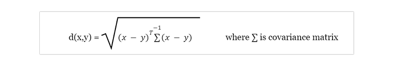
5. Mahalanobis Distance Matrix: 

The Mahalanobis distance matrix is a widely used statistical tool in machine learning and data analysis. This matrix measures the distance between two points in a multi-dimensional space, considering the covariance structure of the variables. It is beneficial when dealing with datasets with highly correlated variables or different measurement scales. For example, it can be used to identify outliers or clusters within a dataset and for classification and prediction tasks. A study by Li et al. (2017) applied this technique to predict customer churn in telecom companies based on various demographic and usage-related features. The authors found that incorporating Mahalanobis distances improved model performance compared to traditional Euclidean distances alone. Overall, the Mahalanobis distance matrix provides valuable insights into complex datasets and helps researchers make more accurate predictions and decisions based on their data analysis results.

Uses For K Nearest Neighbor Algorithm In Machine Learning

Applications outside classification have used the k-NN technique. Some examples of such applications are:

1. Preprocessing of Data: The K-nearest neighbor method may impute missing values in datasets, which is a common occurrence given the prevalence of missing data.
2. Recommendation Engines: The K-nearest neighbor  algorithm has been used to automatically propose more material to consumers based on their clickstream data from websites. Based on the findings of this study (link takes you off of IBM's site), we know that users are classified into groups and then provided suggestions according to the preferences of their cohort. However, this strategy may not be ideal for bigger datasets due to k nearest neighbors scaling difficulties.
3. Healthcare Sector: K-nearest neighbors have also found use in the healthcare sector, where it has been used to forecast the likelihood of events like heart attacks and prostate cancer. The method can function by estimating the probabilities of various gene expressions.
4. Patter Recognition: K-nearest neighbors have been useful in pattern recognition, where it has been used for problems like the categorization of numbers and texts (link resides outside of ibm.com). This has been very useful for deciphering handwritten numbers seen on forms and envelopes.

KNN Model Implementation

KNN (K Nearest Neighbors) is a popular machine learning algorithm for classification and regression tasks. The implementation process of the k nearest neighbors model involves selecting an appropriate value of k, which represents the number of nearest neighbors to consider when making predictions. This value can be determined through cross-validation or other techniques. Once the optimal value of k has been selected, the dataset is split into training and testing sets, with the former used to train the model and the latter utilized to evaluate its performance. During prediction, new data points are compared against existing ones to find their nearest neighbors according to some distance metric such as Euclidean distance or Manhattan distance. Finally, these neighbors are weighted based on their proximity before being used to predict the target variable. Implementing a k nearest neighbors model requires careful selection of hyperparameters and attention paid towards choosing an appropriate distance metric that works well with your specific dataset.

Advantages k Nearest Neighbor Algorithm

• Algorithm’s ease of use and high accuracy, the logistic regression technique is often one of the first classifiers taught to aspiring data scientists.
• The method is flexible because it can quickly adapt to new information as it is introduced, as all training data is kept in memory.
• The Low number of hyperparameters compared to other machine learning algorithms; k nearest neighbor just needs a k value and a distance metric.

Drawbacks of  K Nearest Neighbors Algorithm

• It Does not Scale Well: k nearest neighbor is more space- and memory-intensive than alternative classifiers since it is inefficient. This may require a lot of effort and expense. Increases in memory and storage space have a multiplicative effect on the cost of running a firm and processing more data can lengthen processing times. Although data structures like Ball-Tree were developed to combat computational inefficiencies, the best classifier to use depends on the nature of the underlying business problem.

• Struggles with High-Dimensional Data Inputs: Because of the curse of dimensionality, the k-nearest neighbor method often struggles to deal with high-dimensional data inputs, limiting its usefulness. After the algorithm reaches the ideal number of features, adding more features increases the number of classification mistakes, especially when the sample size is small. This is frequently referred to as the peaking phenomenon.

• Prone to Overfitting: Due to the "curse of dimensionality," k nearest neighbor is also more prone to overfitting. Not only may the choice of k affect the model's behavior, but so can feature selection and dimensionality reduction strategies for avoiding this problem. Overfitting the data can occur at low k values, whereas smoothing down the prediction values by averaging them across a larger region occurs at high k values. On the other hand, underfitting can occur if k is set too high.

Data Science Training For Administrators & Developers

• No cost for a Demo Class
• Industry Expert as your Trainer
• Available as per your schedule
• Customer Support Available

Enroll for Demo Class

Conclusion

K-nearest neighbor (KNN) algorithm is one of the simplest yet most powerful classification algorithms used in machine learning. It works by finding the k number of training samples closest to a new test sample and then predicting its class based on these nearest neighbors' labels. Its main advantage lies in its ability to handle complex decision boundaries without making assumptions about them beforehand. It allows us to specify various hyperparameters such as the number of neighbors (k), distance metric, weights function, etc., which can significantly affect model performance. You can learn more about the k nearest neighbor algorithm and other data science concepts with our data science certification guide and boost your career in data science career path.