Chameleon Hierarchical Clustering Algorithm Using Dynamic Modeling

Chameleon is a highly sophisticated algorithm that has been developed to solve one of the most significant challenges in data science - clustering large and complex datasets. The traditional methods for clustering data, such as k-means or hierarchical clustering, become inefficient when the number of features or dimensions increases. Moreover, these methods often require prior knowledge about the nature of clusters and may not be suitable for dynamic datasets. For an in-depth understanding of the chameleon algorithm, our Data scientist course online helps you explore more about the chameleon clustering algorithm and data mining, the most effective tool of data science.

Chameleon Hierarchical Clustering Using Dynamic Modeling

Chameleon is a hierarchical clustering method that uses dynamic modeling. With its assistance, a calculation is made to determine the degree of similarity between the two groups. Chameleon is used to determine the degree of cluster resemblance.

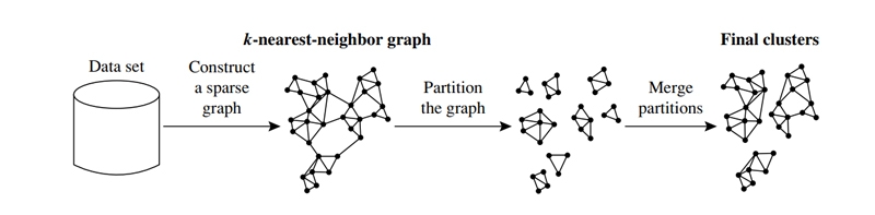
Depends on (1) how near together clusters are located and (2) how closely items inside a cluster are connected to one another. To restate, two clusters are merged into one when the degree to which they are related and their proximity to one another in geographic terms are both significant. Because of this, Chameleon has the ability to automatically adapt to the one-of-a-kind characteristics of the clusters that are being merged and do so without requiring a preconceived model from the user. The merge technique is universal in the sense that it may operate with any data type for which it is possible to create a similarity function. As a result, the process of locating natural and consistent clusters is simplified by using the merge approach. The k-nearest-neighbor approach is what Chameleon uses to construct its sparse graph.

Process of Chameleon Clustering Algorithm

In this method, each vertex in the graph represents a data object, and an edge is only created between two vertices (objects) if the first object is one of the second object's k-most similar objects. The relative strength of the edges is a reflection of the similarities between the nodes in the graph. Chameleon uses a method called graph partitioning to break the k-nearest neighbor graph into multiple smaller subclusters. This is done in order to decrease the number of edges. that need to be deleted from the graph. To put it another way, the weight of the edges that are lost when cluster C is cut in half can be minimized by first dividing it into two smaller clusters, Ci and Cj. It is an examination of the degree to which clusters Ci and Cj are interconnected with one another.

After this, similar subclusters are combined into bigger ones in an iterative manner utilizing an agglomerative hierarchical clustering approach that is utilized by Chameleon. When determining which groups of subclusters are most comparable, the algorithm considers both the physical closeness of the clusters and the connections between them. Chameleon determines the degree of similarity between each pair of clusters Ci and Cj by analyzing the degree to which they are connected to one another (RI(Ci, Cj)) and how close they are to one another (RC(Ci,Cj)).

The relative interconnection between two clusters, denoted by the symbol RI(Ci, Cj), is defined as the absolute connectivity between those clusters multiplied by the total interconnection between all clusters internal interconnectivity of the two clusters, Ci and Cj. That is, 

RI(Ci, Cj) = EC{Ci,Cj}1 /2 (|ECCi | + |ECCj |)

where EC{Ci, Cj} is the edge cut as previously defined for a cluster containing both Ci and Cj. Similarly, ECCi (or ECCj ) is the minimum sum of the cut edges that partition Ci (or Cj) into two roughly equal parts

The degree of Relative closeness The absolute closeness of Ci and Cj normalized with regard to the internal closeness of the two clusters Ci and Cj is the definition of the relative closeness between them. Different methods exist to quantify the proximity of two clusters. To capture this proximity, several existing techniques zero down on the pair of points containing all the points (or representative points) from Ci and Cj closest to each other. One major shortcoming of these methods is their sensitivity to outliers and noise; they can only use a single pair of points. Therefore, CHAMELEON calculates the average similarity between the points in Ci that are related to points in Cj to assess the proximity of the two clusters. This is because the k-nearest neighbor graph is robust against outliers and noise while providing a reliable estimate of the average strength of the connections between data points that reside in the interface layer between the two sub-clusters.

Remember that the average weight of the connections linking vertices in Ci to vertices in Cj is equal to the average similarity between the points in the two clusters.

It is also possible to quantify the degree to which two clusters are related on the inside, a quality known as Ci. The internal closeness of a cluster can be calculated, for example, as the mean weight of all the connections linking the vertices within the cluster (i.e., edges in Ci). In a hierarchical clustering framework, one may argue that the agglomeration edges employed earlier in the process are more robust than those utilized later. That's why you'll find that the average weight of the edges that make up the internal bisection of Ci and Cj is typically lower than the average weight of all the edges in those groups as a whole. On the other hand, the average weight of these edges is a more reliable measure of the degree to which these groups are connected among themselves. As a result, CHAMELEON calculates the proximity between two clusters, Ci and Cj.

RC(Ci ,Cj) =SEC{Ci ,Cj } CiCi+CjSECci+CjCi+CjSECCj

where SEC{Ci, Cj } is the average weight of the edges that connect vertices in Ci to vertices in Cj, and SECCi (or SECCj ) is the average weight of the edges that belong to the mincut bisector of cluster Ci (or Cj)

Phases of Chameleon Clustering Algorithm

When each cluster has a big enough number of vertices, the dynamic framework mentioned may be used to model the similarity between clusters (i.e., data items). This is because CHAMELEON must first calculate each cluster's internal interconnectivity and closeness before determining the relative interconnectivity and closeness of clusters. Both of which are imprecise to compute for clusters with few observations. Consequently, CHAMELEON employs a two-stage algorithm to accomplish its goals. The initial step is to divide the data into several smaller clusters, each of which should have enough information to be dynamically modeled. In the second stage, we'll use the dynamic modeling framework to combine these sub-clusters hierarchically in order to find the true clusters in the data set. Below, we detail the algorithms employed throughout these two stages of CHAMELEON's operation.

Phase 1: 

Identifying Primary Clusters By employing a graph partitioning technique to divide the data set's k-nearest neighbor graph into several smaller partitions, CHAMELEON may quickly identify the first set of sub-clusters by minimizing the edge cut, or the total weight of the edges that cross over into other partitions. As the similarity between data points is represented by edges in the k-nearest neighbor graph, a partitioning that reduces the number of edges in the graph reduces the association (affinity) between the data points in each partition. The theory behind this predicts that there would be more and stronger connections between nodes inside a cluster than between nodes. As a result, there is a strong correlation between pieces of data inside the same partition.

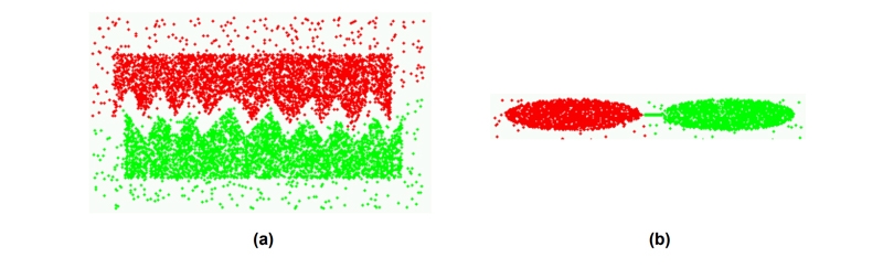
Recently, the multilevel paradigm has been used to construct quick and accurate algorithms for graph partitioning. Extensive studies on graphs occurring in a wide variety of application fields have revealed that multilevel graph partitioning algorithms are particularly successful at capturing the global structure of the graph and capable of finding partitionings that have a very tiny edge-cut. Because of this, they are highly efficient at locating the intrinsic borders of clusters when applied to the k-nearest neighbor graph for partitioning. A multilevel graph partitioning technique applied to the k-nearest neighbor graphs of two geographical data sets yielded the two groups depicted. This diagram clearly demonstrates the efficiency of the partitioning algorithm in locating the low-density dividing zone in the first case and the tiny linking region in the second.

HMETIS is used in CHAMELEON to split a cluster Ci into two sub-clusters, CA I, and CB I, with a minimum edge-cut and at least 25% of Ci's nodes. This third criterion, balance constraint, is essential to finding sub-clusters via graph partitioning. hMETIS can identify an edge-cut-minimizing bisection under balancing limitations. hMETIS may disrupt a natural cluster due to this balancing restriction.

CHAMELEON generates the initial sub-clusters. It starts with all clustered points. It then repeatedly bisects the greatest sub-cluster from the current set using hMETIS. When the bigger sub-cluster has MINSIZE vertices, this operation ends. MINSIZE determines initial clustering solution granularity. MINSIZE should be lower than the average cluster size in the data collection. MINSIZE should be large enough that most sub-clusters have enough nodes to evaluate their interconnectivity and proximity objectively. MINSIZE set to 1%–5% of the data points worked well for most data sets.

Phase 2: 

Dynamic Framework, Merging Sub-Clusters CHAMELEON, uses agglomerative hierarchical clustering to join these tiny sub-clusters once the partitioning-based method of the first phase finds a fine-grain clustering solution. Finding the most comparable sub-clusters is the crucial stage of the agglomerative hierarchical algorithm.

CHAMELEON's agglomerative hierarchical clustering method uses the dynamic modeling framework to find the most comparable clusters by comparing their interconnectivity and proximity. Various approaches to creating an agglomerative hierarchical clustering algorithm consider both metrics. CHAMELEON uses two schemes: The first technique combines only cluster pairings whose relative interconnectivity and relative closeness are over some user-specified threshold TRI and TRC, respectively. CHAMELEON visits each cluster Ci and examines if any of its surrounding clusters Cj match the following two conditions: RI(Ci, Cj) < TRI and RC(Ci, Cj) < TRC. (3)If more than one nearby cluster meets the aforementioned characteristics, CHAMELEON merges Ci with the cluster having the highest absolute interconnectivity, i.e., Cj. After each cluster has had the chance to merge with an adjacent cluster, the desired combinations are executed, and the procedure is repeated. Unlike hierarchical clustering algorithms, this technique merges many pairings of clusters at every iteration. Controlling cluster traits with TRI and TRC.

TRI controls cluster item interconnectivity variability. TRC controls cluster item similarity homogeneity. CHAMELEON's merger process may stop if none of the nearby clusters meet the TRI and TRC requirements. We may either stop the procedure and output the present clustering or try to merge more pairs of clusters by incrementally relaxing the two parameters, perhaps at different rates.The second CHAMELEON strategy merges the pair of clusters that optimize a function that combines relative interconnectivity and relative proximity. Since our aim is to combine couples with high relative interconnectivity and proximity, a logical method to define such a function is to take their product. Merge the clusters Ci and Cj that maximize RI(Ci, Cj) / RC (Ci, Cj). This formula values both parameters equally. We typically choose clusters that favor one of these two measurements. CHAMELEON chooses the pair of clusters that maximizes RI(Ci, Cj) < RC(Ci, Cj) α, where α is a user-specified value. CHAMELEON gives the relative proximity more weight if the number is > 1, and the relative interconnectivity is given more weight when the number is 1. We simply utilized this second method to produce the hierarchical clustering dendrogram in the experimental findings.

Limitation In Chameleon

Chameleon models is a machine learning algorithms that can adapt to different environments or datasets. They are instrumental when dealing with complex and heterogeneous data sources as they can adjust their parameters dynamically based on the input data. This flexibility enables them to perform well in diverse settings across various industries, including healthcare, finance, retail, and more.

However, this adaptability comes at a cost- chameleon models have a higher risk of overfitting than other types of models. Overfitting occurs when the model becomes too specialized in fitting the training dataset but performs poorly on new or unseen data points. In other words, it memorizes the training dataset instead of generalizing patterns within it.The challenge with chameleon models is that they may be highly accurate during initial testing stages where they only encounter similar data distributions as seen during training- but fail spectacularly when exposed to unseen situations or edge cases outside its domain expertise later on.Overcoming these limitations associated with chameleon models' overfitting tendencies while maintaining their flexibility benefits require careful attention by practitioners working in this space.

One solution is implementing regularization techniques such as L1/L2 regularization or dropout layers into neural networks, which penalize model complexity by adding constraints on weights values distribution, thus reducing over-reliance on specific features, ultimately leading to better generalization performance across multiple domains without significantly sacrificing accuracy levels.Another approach would be introducing ensemble methods such as bagging/boosting that combine multiple weak learners into one strong learner capable of handling diverse scenarios robustly while avoiding over-fitting issues commonly observed among single-model architectures like Chameleons aforementioned previously above here!

Data Science Training

• Personalized Free Consultation
• Access to Our Learning Management System
• Access to Our Course Curriculum
• Be a Part of Our Free Demo Class

Sign Up Now

Conclusion

Although chameleon models are highly flexible, their overfitting tendencies can limit their performance in real-world applications. However, by applying regularization techniques or ensemble methods, practitioners can improve model accuracy and reliability while maintaining the flexibility benefits of chameleon models. As data science continues to evolve, it's essential to keep exploring new approaches and refining existing ones to overcome challenges like chameleon models' limitations and further advance this field's growth potential. Understanding Chameleon clustering in data mining begins with understanding data science; you can get an insight into the same through our online certification training courses.