What is Multidimensional and Mutltilevel Association Rule in Data Mining?

This article delves into techniques for mining in a multi-layered, multi-dimensional space, utilizing both multilevel association rule in data mining and multidimensional association rule. It covers the discovery of unusual and negative patterns, as well as multilevel connections and multidimensional correlations. In the case of pattern mining multilevel relations, diverse levels of abstraction are linked together. At the same time, multidimensional relationships involve multiple dimensions or predicates (e.g., linking customers' purchase behavior to their age). Quantitative association rules can be created by assigning numbers as characteristics, with values with a predetermined hierarchy, such as age. Uncommon patterns refer to infrequent yet unique item combinations, while negative correlations between objects are also examined. Understanding multilevel association rules in data mining begins with understanding data science; you can get an insight into the same through our Data Science Training.   

Association Rule in Data Mining

Strong correlations can be found at high levels of abstraction, even with great support; nonetheless, for many applications, these correlations can be regarded as common sense. There is a possibility that we will need to delve much farther into the data to recognize patterns that are genuinely one of a kind.

On the other hand, there may be many patterns at elementary abstraction levels, many of which are trivializations of patterns at higher degrees of abstraction. Consequently, it is fascinating to contemplate how to construct effective algorithms for mining patterns across a wide range of abstraction levels while ensuring that these algorithms have adequate flexibility to permit easy travel between these areas.

Example of Association Rule in Data Mining

You can make data more generalizable by replacing certain instances of low-level concepts with their higher-level concept relatives, also known as ancestors, from a concept hierarchy. This will make the data more generic.

Example:

Let's imagine we have access to the critically crucial collection of sales data from an electronics store, displayed in Table 1. The ideas located at the bottom of an order are the ones that have the least generalization, while the concepts situated at the very top are the ones that are the most particular. 

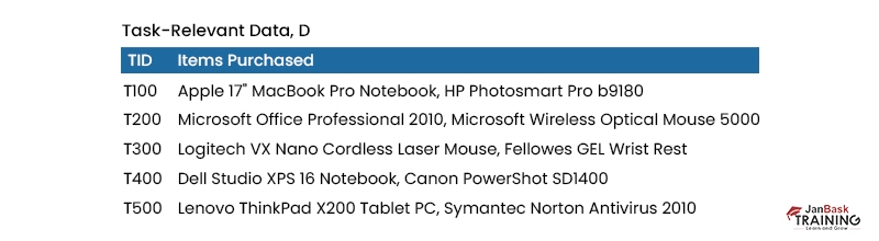
In the order of five levels of concept, representation depicted, "Degree 0" stands for the most fundamental degree of abstraction. The first three levels are considered intermediate degrees of abstraction, while level 4 is considered the most significant level of abstraction. In this scenario, level 1 includes items such as computers, software, printers, cameras, and other computer accessories; level 2 includes laptops and desktops, as well as office and antivirus software; and level 3, includes high-end brands such as Dell desktops, Microsoft office software, and other similar products. Considering this hierarchy, the level 4 abstraction represents the most feasible detailed level. The numbers that are contained in the raw data have been incorporated.

Nominal attribute concept hierarchies are typically already present in the database schema. They can be automatically constructed with techniques such as those outlined. Data on product requirements were used to create the concept hierarchy for our example. Many discretization techniques were discussed to develop concept hierarchies for numeric characteristics. Users familiar with the data, like store managers in our example, may also provide idea hierarchies.

Finding engaging purchasing trends with such raw or basic data is challenging. Finding significant correlations with specific goods might be difficult if they occur in a tiny percentage of transactions, such as the "Dell Studio XPS 16 Notebook" or the "Logitech VX Nano Cordless Laser Mouse." Due to low expected group buying, this bundle is unlikely to reach critical mass.

In contrast, we anticipate that it is simpler to discover robust correlations between broad categories of these things, such as "Dell Notebook" and "Cordless Mouse."

Multilevel Association Rule Mining 

Many-level, or multilevel, association rules are a type of association rule developed via data mining at multiple abstraction levels. Rules of the association at several levels are mined effectively by employing idea hierarchies inside a support-confidence framework. Frequent item sets are often calculated using a top-down approach, where counts are amassed for each idea level from the most general to the most particular, and so on, until no more frequent item sets can be identified. For each tier, you can use Apriori or any other method for finding frequently occurring item sets.

Methods for Association Rule Mining: 

What follows is a discussion of many alternatives to this method, each of which requires "playing" with the support threshold somewhat differently. Nodes represent things or item sets that have been investigated, and nodes with thick margins represent items or set examinations that have occurred often.

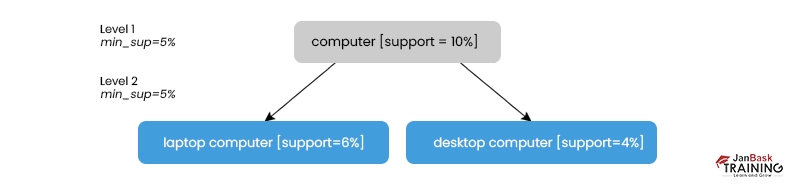
We have uniform support by providing the same amount of backing across the board.

• Minimal Support Criterion Method

Mining at each level of abstraction uses the same minimal support criterion.

A minimum support requirement of 5% is applied (for mining from "computer" down to "laptop computer"). The terms "computer" and "laptop computer" are standard, whereas "desktop computer" is rarely used.

Using a standard minimum support level can streamline the search process. The process is extremely straightforward because consumers need minimal support from only one. Given that every ancestor is a superset of its descendants, we may use an Apriori-like optimization strategy:

The search will ignore any item for which the ancestors do not have minimal support.

Despite its popularity, the uniform support method has its challenges. Products with a greater degree of abstraction are more likely to appear frequently than those with a lower level of abstraction. Because of this, it's essential to find a happy medium between setting the minimum support threshold high enough to catch all but the most vital links and making it too low to miss any significant ones. Too low of a point might cause the generation of numerous irrelevant linkages at very high abstraction levels.

• Reduced Support Method

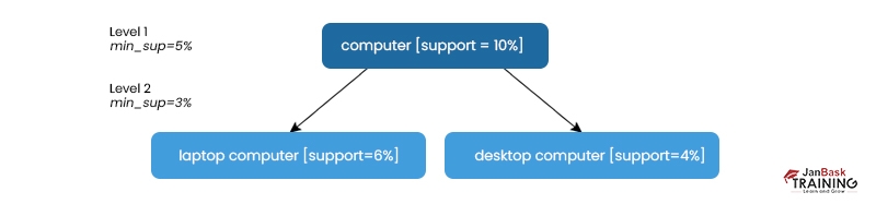
This is the impetus for the following strategy. Through the use of lower levels of minimal support (hence referred to as "reduced support"):

A lower threshold of support is required at lower levels of abstraction. The threshold is lower at higher levels of abstraction. The above figure shows that 5% and 3% minimum support are required for levels 1 and 2, respectively. Computer, laptop computer, and desktop computer are all examples of common noun phrases here.

Building up user-specific, item- or group-based minimal support levels may be preferable when mining multilayer rules, as users or experts typically have insight into which groups are more significant than others. Set minimum support levels depending on the product price or items of interest; for instance, pay special attention to the association patterns, including those categories (such as "camera with price over $1000" or "Tablet PC") and the system will prioritize such patterns.

The threshold is often set to the lowest value among the participating groups for mining patterns containing elements from many groups with varying support thresholds. This way, useful patterns comprising elements from the least-supported group won't be filtered out. Meanwhile, it's important to maintain the minimum required level of support for each group to prevent the accumulation of boring collections of things from any group. After the itemset mining, different metrics of interestingness may be applied to draw out the most pertinent rules.

When mining under limited or group-based support, remember that the Apriori attribute does not always hold evenly across all objects. On the other hand, effective strategies may be created by expanding the property. 

As a negative byproduct of the "ancestor" relationships among things, pattern mining multilevel association rules generates numerous duplicate rules across several abstraction levels. Using the idea hierarchy, one can see that the "laptop computer" is the progenitor of "Dell laptop computer," prompting us to evaluate the following rules:

Clients who made purchases in AllElectronics transactions are represented by the variable X

Support = 8%, Confidence = 70% buys(X, "laptop computer") > buys(X, "HP printer").
compare('buys(X, 'Dell laptop computer') > compare('buys(X, 'HP printer')] [support = 2%, confidence = 72%] give something new or different?" We should eliminate the latter, less broad rule if it doesn't add anything to the conversation. Let's consider some possible methods of determining this. If the items in R2 can be acquired by replacing them with their predecessors in a concept hierarchy, then R2 is an ancestor of R1.

The reason is that "laptop computer" predates "Dell laptop computer." This definition suggests that a rule is redundant if its support and confidence are near the "anticipated" values based on a rule's parent.

Multidimensional Associations Rule in Data Mining 

Association rules with a single implying predicate, such as "buys," have been the focus of our attention so far. The Boolean association rule buys(X, "digital camera") buys(X, "HP printer"), for instance, may be found by mining our AllElectronics database.

Each unique predicate in a rule is referred to as a dimension, in keeping with the terminology  used in multidimensional databases. Thus, the Rule is a single-dimensional or intra-dimensional association rule since it has a single distinct predicate (such as buys) with multiple occurrences (i.e., the predicate appears more than once within the rule). Rules like this may often be extracted from transactional data. You can learn more about six stages of data science processing to grasp the above topic better.

When analyzing sales and related information, it's not uncommon to combine it with relational data or include it in a data warehouse rather than relying just on transactional data. Multidimensionality is a hallmark of such data warehouses. For instance, a relational database may store additional information linked with sales transactions outside just the things purchased.

Associated with the goods and the deal itself, including the description of the goods or the location of the sale's branch. A customer's age, profession, credit score, income, and address are all examples of relational data that may maintain with what they bought. To mine multi-predicate association rules like age(X, "20-29"), occupation(X, "student") purchases(X, "laptop"), we must treat each database attribute or warehouse dimension as a predicate.

Multidimensional association rules are those that involve three or more dimensions or predicates. The rule has three unique predicates: age, occupation, and purchases. For this reason, we may confidently declare that it contains no recursive predicates. Interdimensional association rules span many dimensions but have no common predicates. Multi-dimensional association rules with repeated predicates can also be mined for helpful information. These rules have predicates that appear more than once. Hybrid-dimensional association rules are a term for these types of guidelines. For instance, consider the rule age(X, "20...29") > buys(X, "laptop") > buys(X, "HP printer"), where each iteration of the predicate buys is applied to a different X.

Attributes in a database can be either nominal or quantitative. Nominal attributes (categorical attributes) have "names of objects" as their values. There is no hierarchy among the potential values for nominal properties (e.g., occupation, brand, color).Age, salary, and cost are all examples of quantitative qualities, implying a hierarchy of relative importance. 

Multidimensional Association Rules in Data Mining Can be Divided Into Two Broad Camps Based on Quantitative Features: 

• One method involves leveraging existing idea hierarchies to discretize quantitative features. There is a discretization step before mining. In the case of income, for instance, interval labels such as "0..20K," "21K..30K," "31K..40K," and so on can be used in place of the original numeric values of this attribute thanks to a concept hierarchy. The present case involves a fixed and specified discretization.The interval labels on the discretized numeric attributes allow them to be interpreted as nominal attributes (where each interval represents a category). Using a static discretization of quantitative characteristics, we refer to this as mining multidimensional association rules.

• The second method divides quantitative characteristics into discrete groups, or "bins," according to how the corresponding data is distributed. During the mining process, these containers may be mixed together again. For example, a dynamic discretization procedure has been devised to maximize the reliability of the rules mined. Association rules discovered using this method are sometimes known as (vibrant ) quantitative association rules. Then numerical attribute values are treated as quantities rather than as established ranges or categories. Let's look into each of these methods for mining MDA rules.

So as not to get too complicated, we will only be talking about the laws of the relationship between dimensions. In multidimensional association rule mining, we look for frequent predicate sets rather than regular, frequent item sets, as in single-dimensional association rule mining. A set with k conjunctive predicates is called a k-predicate set in set theory. For example, Rule's set of predicates "age, occupation, buys" is a 3-predicate set.

Data Science Training

• Personalized Free Consultation
• Access to Our Learning Management System
• Access to Our Course Curriculum
• Be a Part of Our Free Demo Class

Sign Up Now

Conclusion

Pattern mining in multilevel, multidimensional space is a powerful technique that can provide valuable insights for businesses looking to extract meaning from complex datasets. By combining the concepts of multilevel and multidimensional association rules, businesses can gain a more comprehensive understanding of their data and identify patterns that might otherwise go unnoticed. As datasets continue to grow in complexity, this technique will become increasingly important for organizations seeking competitive advantages through a better understanding of their customer's behaviors. You can also learn about neural network guides and python for data science if you are interested in further career prospects in data science.