How to Work with Regression based Models?

What are Regression Models?

Regression analysis means to contemplate the connection between one variable, generally called the dependent variable, and a few different factors regularly called the independent variable. Regression analysis extends from linear to nonlinear and parametric to nonparametric models. Regression analysis is a mathematical way of sorting out which variable is efficient. Independent variables are the variables that have an impact on the dependent variables.

                                           

The blue line in the graph is the regression line which shows the relationship between independent and dependent variables.

Usage of the Regression Model in companies:

1. Regression models are highly used in companies for analytics for making smart decisions.
2. Most companies use regression models to explain the processes to their customers for a better understanding of the customer.
3. Another use of these models is to predict about future so that decision making for prospects is easy.

Regression-based models

Linear Model

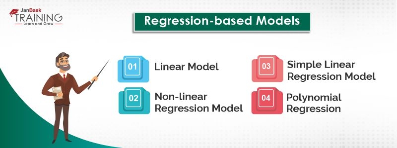
The linear regression model can be explained as a linear relationship made between dependent and independent variables. The model with one variable is known as a simple linear model and a model with more than one variable is known as a non-linear regression model.

Simple Linear Regression:

A regression model that allows the linear relationship between an independent variable(X) and an independent variable(Y).

The equation for simple linear regression is:

Y= a + bX

Where,

Y - dependent variable
X - independent variable 
b - a slope of the line
and
a - y-intercept.

Non-Linear Regression Model:

When there is more than one independent variable then it is called the Non-Linear Regression Model. The equation for non-linear regression is:

 Y = a0 + b1X12

A nonlinear regression model can have multiple different forms.

Simple linear regression model:

This is a linear model based on a single explanatory variable. It works on two-dimensional points where one is dependent and the other one is an independent variable. The main goal of this regression model is to make the sun of these squared deviations as small as it could be.

Polynomial regression

Polynomial regression is a type of regression examination where the connection between the independent variable x and the dependent variable y is demonstrated as the furthest limit polynomial in x. Polynomial relapse fits a nonlinear connection between the estimation of x and the relating restrictive mean of y, indicated E(y |x). Although polynomial relapse fits a nonlinear model to the information, as a measurable estimation issue it is direct, as in the relapse work E(y | x) is straight in the obscure parameters that are assessed from the information.

Multivariate Regression Model:

It is a statistical linear model.

Y=XB+U 

 Where, 

 Y= Dependent variable 

 X=Independent variable 

 B=Parameters that needs to be calculated 
U=Errors

Moving average model.

The old-style technique for time series decomposition began during the 1920s and was generally utilized until the 1950s. It despite everything structures the premise of many time series decomposition techniques, so it is imperative to see how it functions. The initial phase in an old-style decomposition is to utilize a moving normal technique to gauge the pattern cycle, so we start by examining moving midpoints.

yt=c+εt+θ1εt−1+θ2εt−2+⋯+θqεt−q,

Where εt is white noise.

Moving averages of moving averages

It is conceivable to apply a moving normal to a moving normal. One explanation behind doing this is to make an even-request moving normal symmetric. Different mixes of moving midpoints are additionally conceivable.

Weighted moving averages

Mixes of moving midpoints bring about weighted moving midpoints. A significant favourable position of weighted moving midpoints is that they yield a smoother gauge of the pattern cycle. Rather than perceptions entering and leaving the computation at full weight, their loads gradually increment and afterwards gradually decline, bringing about a smoother bend.

Differencing

Differencing is computing the differences between consecutive observations. It is used for stabilizing the mean of a time-series by removing the change obtained in its level and eliminating the seasonality obtained from the time-series. Differencing comes into an application where the provided data has one less data point than the original data set.

For instance, given a time-series Xt, one can create a new series Yi = Xi - Xi-1 As well as its general use in transformations, differencing is mostly used in time series analysis. 

Types of differencing.

Random walk model.

differencing is the change between consecutive observations in the original time-series, can be written as:

Y’t = Yt – Yt-1

series have (t-1) values only. When white noise observed in the particular differenced series then it will be rewritten as:

Yt − Yt-1= εt

εt denotes white noise. After rearranging we get:    

Yt = Yt-1 + εt.

This model is mainly used for non-stationary data and economic or financial data. Because future movements by this differencing model are unpredictable so forecasting results obtained using this model is equivalent to the last observation of the model.

Second-order differencing.

Most of the times the differenced data will not appear to be stationary and it is necessary to perform the second-order differencing to obtain a stationary series.

y′′t = y′t −y′t−1

 = (yt−yt−1) − (yt−1−yt−2)

 = yt−2yt−1+yt−2.

Second-order differencing the series will have T−2 values. In practice, it is never necessary to go beyond second-order differences.

Seasonal differencing.

Seasonal differencing is needed to be performed in the same season than in that case, seasonal differencing is used. It calculates the difference between consecutive observations of the same season.

y′t = yt – yt-m

where m= the number of seasons. These are also called “lag-mm differences”. The results which are forecasted from the seasonal differencing model are equivalent to the last observation from the relevant season.

Simple exponential smoothing.

Simple exponential smoothing is a powerful time-series forecasting method for data which do not have a particular trend or any seasonality. It is also known as single exponential smoothing.

The formula for simple exponential smoothing is:

St = αyt-1 + (1 – α) St-1

Where: t = time period.

α = the smoothing constant, its value ranges from 0 to 1. Now, when the value of α is approximate to zero, smoothing occurs more slowly. Following this, the best suitable value for α is the one which results in the smallest mean squared error (MSE). The number of ways exists to perform this, but one of the most popular methods is the Levenberg–Marquardt algorithm.In case of simple exponential smoothing, exponential functions are used for exponentially decreasing weights as compared to simple moving average in which past observed values are weighted equally.

Conclusion

It is very difficult to conclude the regression model because of its unclearness. Regression depends upon how data is collected and how it is analyzed. Most important thing is that Is the regression model applied is the best-fit regression model. Regression Analysis is utilized in the more extensive sense; be that as it may, basically it depends on measuring the adjustments in the dependent variable (regressed variable) because of the adjustments in the independent variable by utilizing the information on the dependent variable. This is because all the regression models whether linear or non-linear, simple or multiple relate the dependent variable with the independent factors.

Please leave comments and query in the comment section.

FaceBook Twitter Google+ LinkedIn Pinterest Email