An Easy To Interpret Method For Support Vector Machines

The support vector machine is a machine learning algorithm that follows the supervised learning paradigm and can be used for both classifications as well as regression problems though this is primarily a classification algorithm. This algorithm primarily works by designing the hyperplanes and increasing the margin between them.

Introduction Support Vector Machine

In the domain of machine learning, support vector machines belong to the associated learning under the broader domain of supervised learning. These models can be used for classification as well as regression. This algorithm particular belongs to the class of non-probabilistic binary classifiers though under few variations like Platt scaling and allied stuff that these can also be used probabilistic classifiers. Being a binary classifier, SVM owing to its inherent design can only assign the data points to two classes only. A model utilizing SVM maps the data points in space in such a fashion that two classes are separated by a clear gap and are concerned about increasing the gap.

In support vector machines that utilize the n-features for its input, the data items are plotted as a point in N-Dimension space with each feature corresponding to the value of a particular coordinate. Then, we check the class to which it belongs. By the basic definition of SVM, it’s a binary classifier and thus, utilizes the normal XY-coordinate geometry which is depicted in figure 1, below.

Defining a support vector:

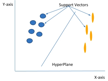
The data points that are close to the hyperplane and have an impact on the position and alignment of the hyperplane are called support vectors. These data points this algorithm to its name as well. The main aim of using a support vector is to increase the functional margin which is introduced with the hyperplane. Changing or removing these datapoints alter the position and orientation of hyperplane as well.

Hyperplane:

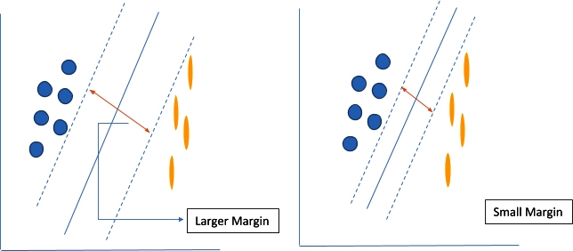
The decision boundaries that help classify the data are called the hyperplanes. Data points that fall on either side of the hyperplane belong to the same class. The number of dimensions to which a hyperplane exists also varies according to the number of features in the input space. If there are only two features in the input space, then the hyperplane is a straight line as shown in Fig. 1. Whereas, if there 3 features then hyperplane is a dimensional plane. For dimensional greater then 3D, it will also exit but the visualization is not possible. The hyperplane generated ios separated from the support vectors with some margin. This margin should be as large as possible. Figure 2 depicts the concept of margin which is technically known as the functional margin and it remains an important concept in support vector machines.

Read: An Ultimate Guide To Python For Data Science (2024)

Cost Function:

The functioning of the support vector machines is all about increasing the margin between the data points and the hyperplane. A loss function named as hinge loss is one of the most commonly used loss function to perform this activity. Mathematically, Hinge loss is given by:

c(x,y,f(x)= f(x)={0,if y*f(x)≥1 1-y*f(x),
else  ……………………………………………………………….(1)
Eq. (1) can also be represented as
c(x,y,f(x))=(1-y*f(x))_+ ………………………………………………………………………………..(2)

If the predicted and the actual value happen to be of the same sign then the cost becomes 0 as evident from figure 1. Scenarios, where they are not zero the calculation of the loss value takes place. In Hinge loss, a regularization parameter is added to balance the margin at maximum separation and bring the loss at a minimum. Once, the regularization parameter is added equation (2), looks like:

〖〖min〗_w λ|(|w|)|^2+∑_(i=1)^n(1-y_i<x_i,w>〗_+…………………………………………………………………….(3)

The derivative of equation(2), can be used to update the weight with the help of the gradient descent algorithm.

Designing models with Support vector machine:

A support vector machine happens to be the type of binary classifier. Thus, by definition, they can be used to classify only 2 classes. But, can also be used for a multi-class classifier. This can be done by manipulating the dataset. If we have 3 classes for classification. Native support vector machines are useless. But instead of saying 3 class, if we say, that every class is a negation of its own class then we can have 3 classifiers for saying are they that class or not. IN this way, support vector machines can also be used for multi-class classification. The number classifier trained in this case is

(n*(n-1))/2 ……………………………………………………………………………………………………………………..(4)

Thus, the number of classifier increase but the model is able to handle the multiclass data. This function comes in hand with sklearn as SVC.

In this section, python is utilized with its sklearn library. Different SVM based classifiers will be demonstrated over an iris dataset. Details of the iris dataset can be found here.

Read: What Is Time Series Modeling? Forecasting Process and Model

Importing the libraries:

import numpy as np
import matplotlib.pyplot as plt
from sklearn import SVM, datasets

The next step is to create the mesh for plotting points:

def make_meshgrid(iris_in, target, h=.02):

    iris_in_min, iris_in_max = iris_in.min() - 1, iris_in.max() + 1
    target_min, target_max = target.min() - 1, target.max() + 1
    vector, label = np.meshgrid(np.arange(iris_in_min, iris_in_max, h),
                         np.arange(target_min, target_max, h))
    return vector, label

Once the mesh is created, the decision  boundries for the classifier are created:

def plot_contours(ax, model, vector, label, **params):
    
    A = model.predict(np.c_[vector.ravel(), label.ravel()])
    A = A.reshape(vector.shape)
    out = ax.contourf(vector, label, A, **params)
    return out

Now, the data set is being imported and 3 classifiers over a 2D space will be created and classifier are trained using a for and plotted:

iris = datasets.load_iris()     #loading the dataset
X = iris.data[:, :2]                  #taking only 2 features as for dimentions greater the 2, visualization won’t  be possible
y = iris.target
C = 1.0  # SVM regularization parameter
models = (svm.SVC(kernel='linear', C=C),  #defining models
          svm.LinearSVC(C=C, max_iter=10000),
          svm.SVC(kernel='poly', degree=3, gamma='auto', C=C))
models = (model.fit(X, y) for model in models)
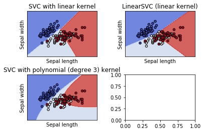
titles = ('SVC with linear kernel',
          'LinearSVC (linear kernel)',
          'SVC with polynomial (degree 3) kernel')
fig, sub = plt.subplots(2, 2)    #defining the plots and plots 2*2 = 4 grid
plt.subplots_adjust(wspace=0.4, hspace=0.4)

X0, X1 = X[:, 0], X[:, 1]
xx, yy = make_meshgrid(X0, X1)
for models, title, ax in zip(models, titles, sub.flatten()):
    plot_contours(ax, models, xx, yy,
                  cmap=plt.cm.coolwarm, alpha=0.8)
    ax.scatter(X0, X1, c=y, cmap=plt.cm.coolwarm, s=20, edgecolors='k')
    ax.set_xlim(xx.min(), xx.max())
    ax.set_ylim(yy.min(), yy.max())
    ax.set_xlabel('Sepal length')
    ax.set_ylabel('Sepal width')
    ax.set_xticks(())
    ax.set_yticks(())
    ax.set_title(title)

x=plt.show()

This will produce a grid of 2*2 = 4 grids which will depict the decision boundaries of the classifier trained. One box remains empty as we are using plt.subplot which makes 4 grids as per specifications and there are only 3 classifiers.

Advantages and Disadvantages of Support vector machines:

Advantages:

Read: An Easy To Understand Approach For K-Nearest Neighbor Algorithm

1. It is possible to introduce L2 regularization in the Support vector machines. Thus, helps in prevent over-fitting.
2.  kernel functions can be utilized in the support vector machines to handle non-linearity in the data.
3. Support vector machines can be used for both classifications as well as regression.
4. In the cases of small changes in the support vector machines. The hyper-plane is not impacted much. Resulting in a much stable model.

Disadvantages:

1. While handling non-linear data in support vector machine, it becomes very tricky to select the appropriate kernel function.
2. If the input space consists of N-dimension space with N being sufficiently high, the model will generate a high number of support vector which will impact the training speed.
3. Scaling of features is required before training of the model is done.
4. Space and time complexity for support vector machines is very high.
5. In comparison to viewable models like decision trees, the model generated by support vector machines is difficult to interpret.

End Notes

Support vector machines can produce models that are robust as well as accurate even in scenarios where the input dataset is non-monotonous or is not linearly separable. Thus, they are convenient to use. Since the data is separated linearly, thus they don’t need human expertise for training.  These days there are a number of tools available for implementing support vector machines and these have shown remarkable results in text classification and allied stuff.

Please leave the query and comments in the comment section.

FaceBook Twitter Google+ LinkedIn Pinterest Email