Introduction to Regression Analysis & Its Approaches

Introduction

Regression analysis is an algorithm of machine learning that is used to measure how closely related independent variables relate to a dependent variable. Regression models are highly valuable because they are one of the most common ways to make inferences and predictions. The aim to study regression analysis depends upon the relationship between two variables named as a dependent variable and an independent variable and these are used to make data-driven decisions. The regression models can be of type linear, non-linear, parametric and non-parametric. 

Regression-based models are widely used for forecasting, estimation and also in the interpolation or extrapolation of data. These types of models hence find a great deal of application in Weather prediction, Stock Market, Business Intelligence, etc. Some examples of the regression models are KNN (k-nearest neighbours), multiple linear regression models, logistic regression models, and conventional non-linear regression models. However, the most common regression model is the linear regression, in which the analysts have to draw the line that fits the criterion for a linear mathematical equation. "The method of the least squares" is known to be the earliest form of regression.  

Regression models components:

• Unknown Parameters (can be represented as Scalar or Vector)
• Dependent Variables (Scalar representation is used)
• Independent Variables (Vector representation is used) 
• Error terms (These are not often observed and can be represented as Scalar Terms)

Significance of moving average models- An easy guide

The regression models in their very basic form are just mathematical models that help to solve complex mathematical problems. Therefore, these models may require some assumptions in achieving the results. These assumptions are small but they may lead to some uncertainty which may also lead to false predictions or forecasts. Some analysts came up with the moving average model and the moving average smoothing to deal with this uncertainty or error. A moving average method is a tool for the "Time Series Analysis".

The history of the moving average method goes as early as the 1901s. The initial name given to the method was the "Instantaneous Averages". However, in 1909 the name was changed to "Moving Averages" by R.H. Hooker. 

In the moving average model past forecast errors are used in regression-like models instead of the past values of the forecast. The moving averages can be categorized into two sub-categories:

Read: Deep Learning Tutorial Guide for Beginners

• Centred moving average
• Trailing moving average

The centred moving average models are useful in making the trend more visible whereas the trailing moving average model performs better in the case of forecasting. The two models differ in the placement of the window of the average model. The moving average window with width 'w' means for each set of w consecutive values, the average value is calculated. The only job for the analyst is to determine the value of the 'w'. 

The window size may be specific for each task. For example, if an analyst wants to get the local trends, he would keep the size of the window small while a large window size would be required to get the Global trends. 

The moving average is used to smooth out certain fluctuations in the time-series data and make the cycles more visible. However, while dealing with non timed related data, it just smoothens the data.

Yule, a mathematical researcher explained the implication of the special cases of the moving average method in the difference correlation method. 

Below is a sample of the first 5 rows of the dataset, including the header row describing the number of daily female births in California in 1959.

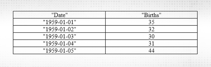
Figure 1: Female Birth Dataset

Read: A Complete Guide for Processing of Data

Code for converting a given “Female Birth Dataset” into moving average:

from pandas import read_csv
from matplotlib import pyplot
set = read_csv('daily-total-female-births.csv', header=0, index_col=0)
alpha = set.alpha(window=4)
alpha_mean = alpha.mean()
print(alpha_mean.head(8))
# plot original and transformed dataset
set.plot()
alpha_mean.plot(color='red')
pyplot.show()

Output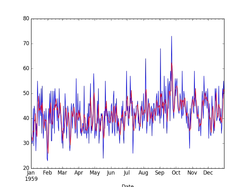 

Figure 2: Moving Average Transform

The raw observations are plotted (blue) with the moving average transform overlaid (red).

Why is differencing crucial for the Time Series Analysis?

Differencing, in simple mathematical terms, is the difference between the two consecutive values. The different method is used to remove a pattern or a trend from the data. In statistical terms, it is a stationary transformation applied to the time-series data. However, sometimes differencing fails to smoothen the data and hence differencing is applied one more time and this is known as Second-order differencing.

It is a pre-processing method used to smoothen or filter the data before forecasting or predicting the data. Trends or patterns are needed to be removed from the non-stationary data to achieve stationary data. This stationary data can be further used to make non-ambiguous predictions. These patterns if not removed may lead to a certain bias which may lead to false or unrelated predictions. Other than trends or patterns, differencing can also be used to remove seasonality which also leads to a certain ambiguity in the results. 

Read: The Best Data Science Projects (Beginner To Advanced)

Simple exponential Smoothing - The best approach for time series analysis

A simple exponential smoothing method produces very similar results as forecasting with the moving average method. This method is much more cost-effective, flexible and easy to use without affecting its performance. The only difference is that instead of a simple average, a weighted average is taken for all the past values. This helps in assigning more weights to the most recent data and at the same time, the old data is not completely ignored. The simple exponential smoothing can also be used upon the stationary data, i.e. data that do not showcase any trend or pattern. Differencing can be applied to the data to get the desired type of data, as mentioned above. The simple exponential smoothing method collects information based upon the difference between the forecast and the past values. This information helps in correcting future predictions. The forecast value is adjusted based on the smoothing factor. 

The simple smoothing factor can be calculated with just the smoothing factor, previous forecast values and past errors in predictions. This helps in saving a lot of storage space and the computation power as well. This is the reason that this method finds its application in the real-time analysis for the time series data. The smoothing factor "α" (alpha) is determined by the user. This value determines the learning rate. If the smoothing factor is closer to 1, it indicates fast learning and if its value is closer to 0, it indicates slow learning. The value of alpha is chosen based upon the amount of smoothing required.

Conclusion

In conclusion, it is safe to say that differencing is required on a time series data to get accurate and redundant free results. Moving average method and the simple exponential smoothing method can only be applied to the stationary data. Both of the methods have factors (Window width and the smoothing factor) which are determined by the user. These factors help in prioritizing the most recent data over the past data. Both methods will result in the same forecasting results if the value of w is two divided by α -1. The simple exponential smoothing methods prove to be a better method due to its cheap computation and optimized storage capabilities.

Please leave the query and comments in the comment section.

Read: A Practical guide to implementing Random Forest in R with example

FaceBook Twitter Google+ LinkedIn Pinterest Email